ggPSE provides ggplot2-based periodic table visualizations. Every function returns a standard ggplot2 object, so you can add themes, annotations, and combine plots with patchwork as usual.
Basic gradient map
Supply a data frame with element symbols and a numeric column.
ggPSE() maps the column to a fill gradient and returns a
standard ggplot2 object.
battery <- data.frame(
  symbol     = c("Li", "Co", "Ni", "Mn", "Fe", "P", "C"),
  importance = c(0.95, 0.88, 0.75, 0.60, 0.45, 0.40, 0.35)
)
ggPSE(battery, value_col = "importance", legend_title = "Battery relevance")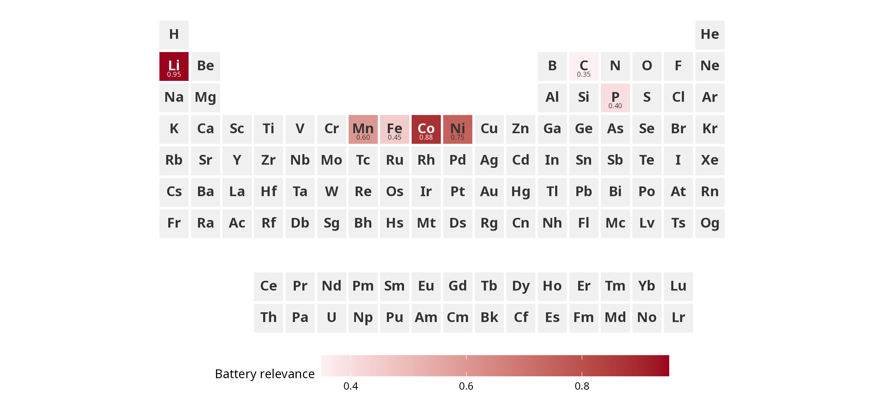
Elements with no data appear in neutral grey. Because the result is a plain ggplot2 object, you can keep adding layers:
ggPSE(battery,
      value_col    = "importance",
      color_low    = "#f7fbff",
      color_high   = "#08519c",
      legend_title = "Battery relevance") +
  labs(title = "Critical elements for Li-ion batteries") +
  theme(plot.title = element_text(size = 11, face = "bold", hjust = 0.5))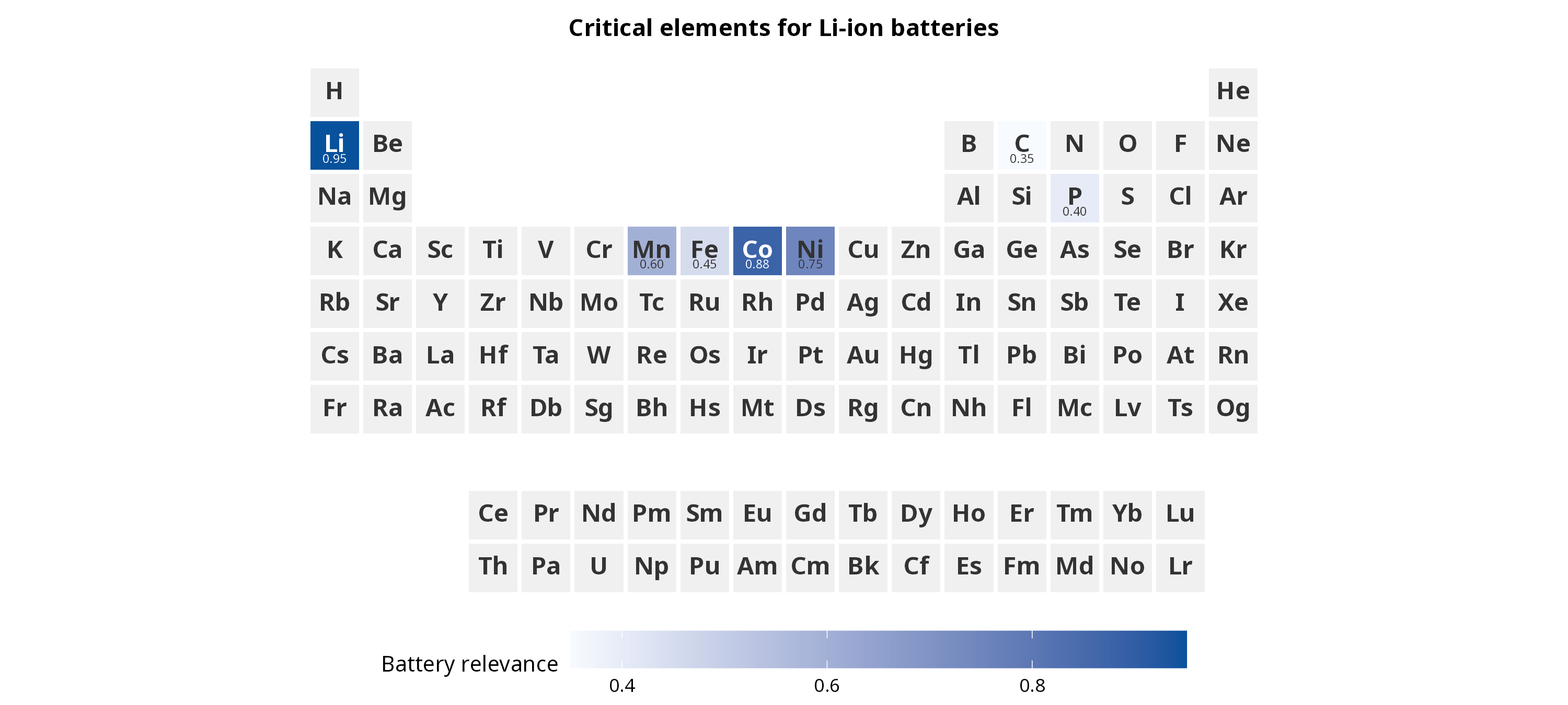
Subsetting the table
Use groups, periods,
lanthanides, and actinides to display only a
portion of the periodic table.
# Transition metals only
ggPSE(battery,
      value_col   = "importance",
      groups      = c(3, 12),
      periods     = c(4, 6),
      lanthanides = FALSE,
      actinides   = FALSE,
      legend_title = "Battery relevance")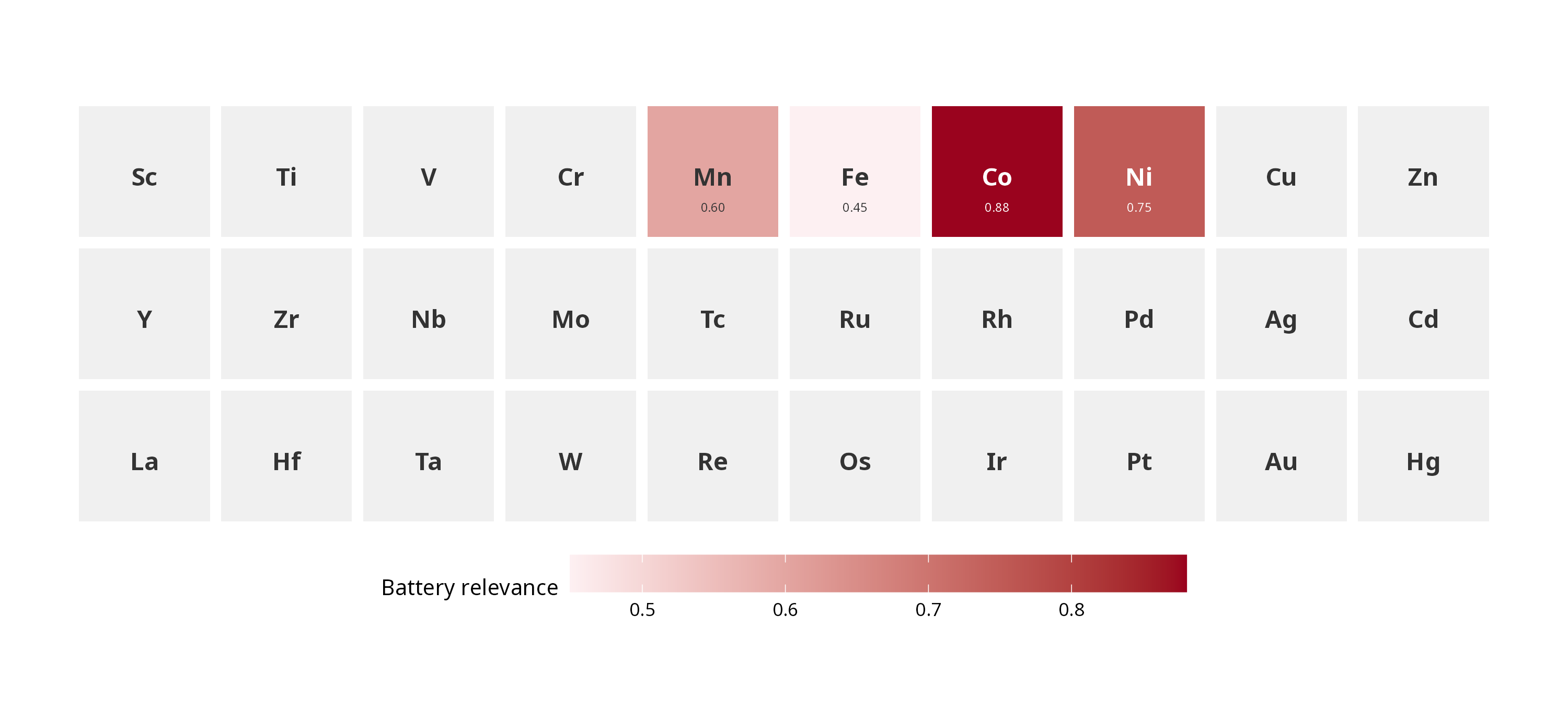
# Full table without lanthanides and actinides
ggPSE(battery,
      value_col   = "importance",
      lanthanides = FALSE,
      actinides   = FALSE,
      legend_title = "Battery relevance")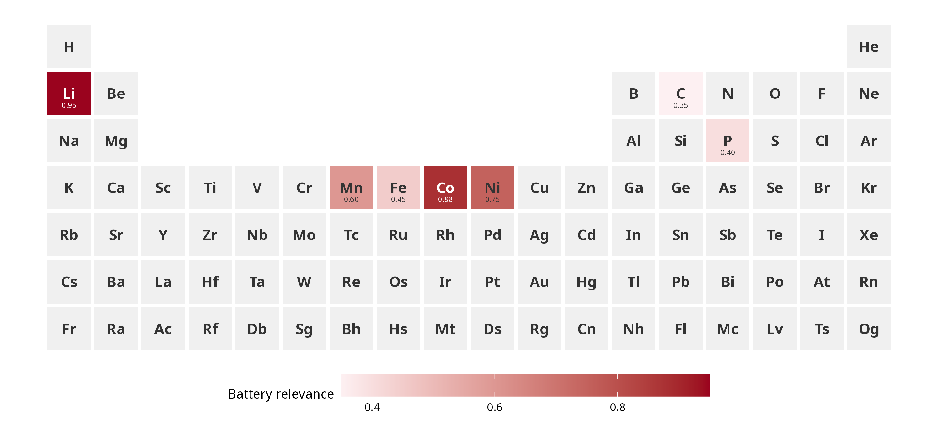
Highlighting element groups
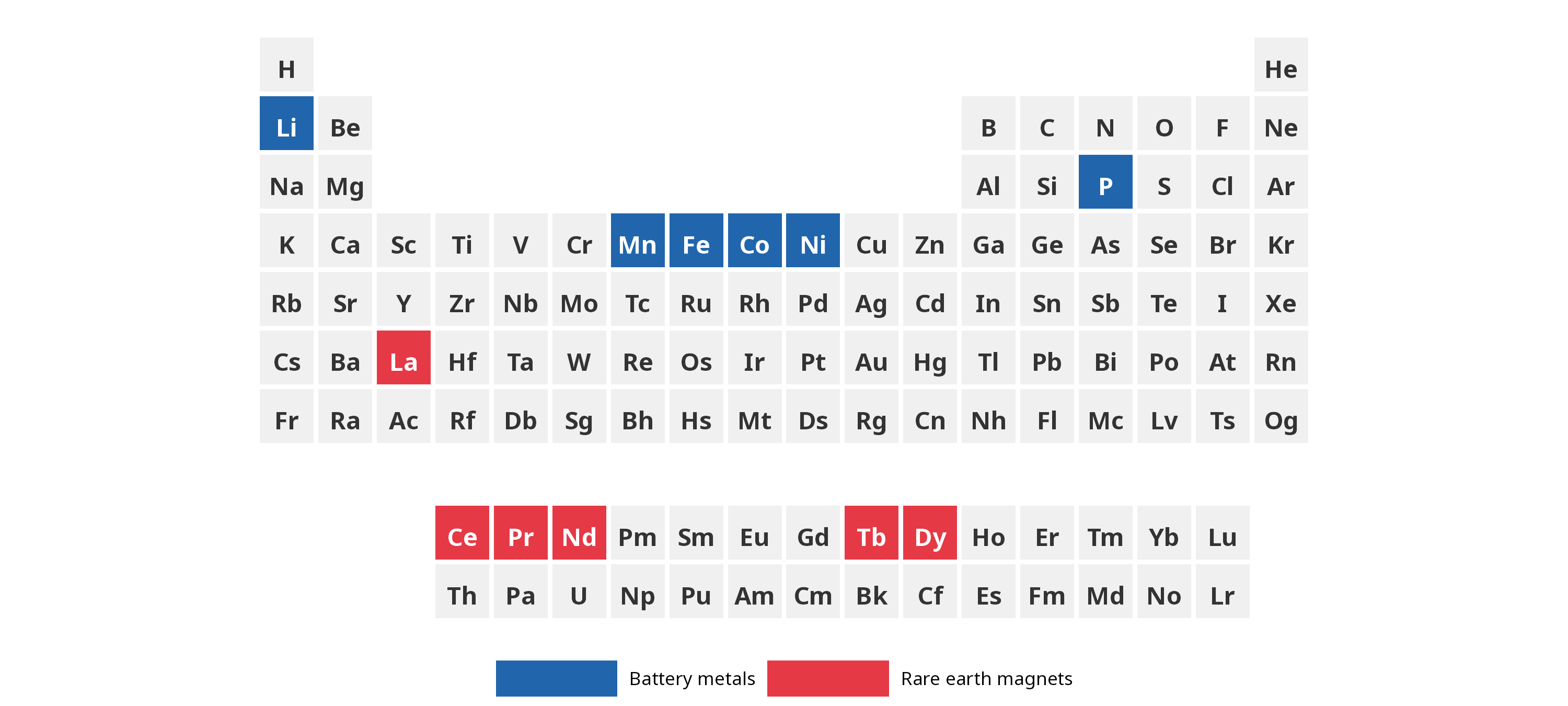
The highlight parameter colors groups of elements and
adds a legend entry for each group.
ggPSE(highlight = list(
  list(symbols = c("Li", "Co", "Ni", "Mn", "Fe", "P"),
       color   = "#2166ac",
       label   = "Battery metals"),
  list(symbols = c("Nd", "Dy", "Tb", "Pr", "La", "Ce"),
       color   = "#e63946",
       label   = "Rare earth magnets")
))
Bubble size encoding
ggPSE_bubble() maps a numeric column to bubble size on a
clean white background.
supply_risk <- data.frame(
  symbol = c("Li", "Co", "Nd", "Dy", "Pt", "Rh", "In", "Ga"),
  risk   = c(0.62, 0.91, 0.84, 0.88, 0.52, 0.70, 0.78, 0.65)
)
ggPSE_bubble(supply_risk, size_col = "risk",
             bubble_color = "#d73027", legend_title = "Supply risk score")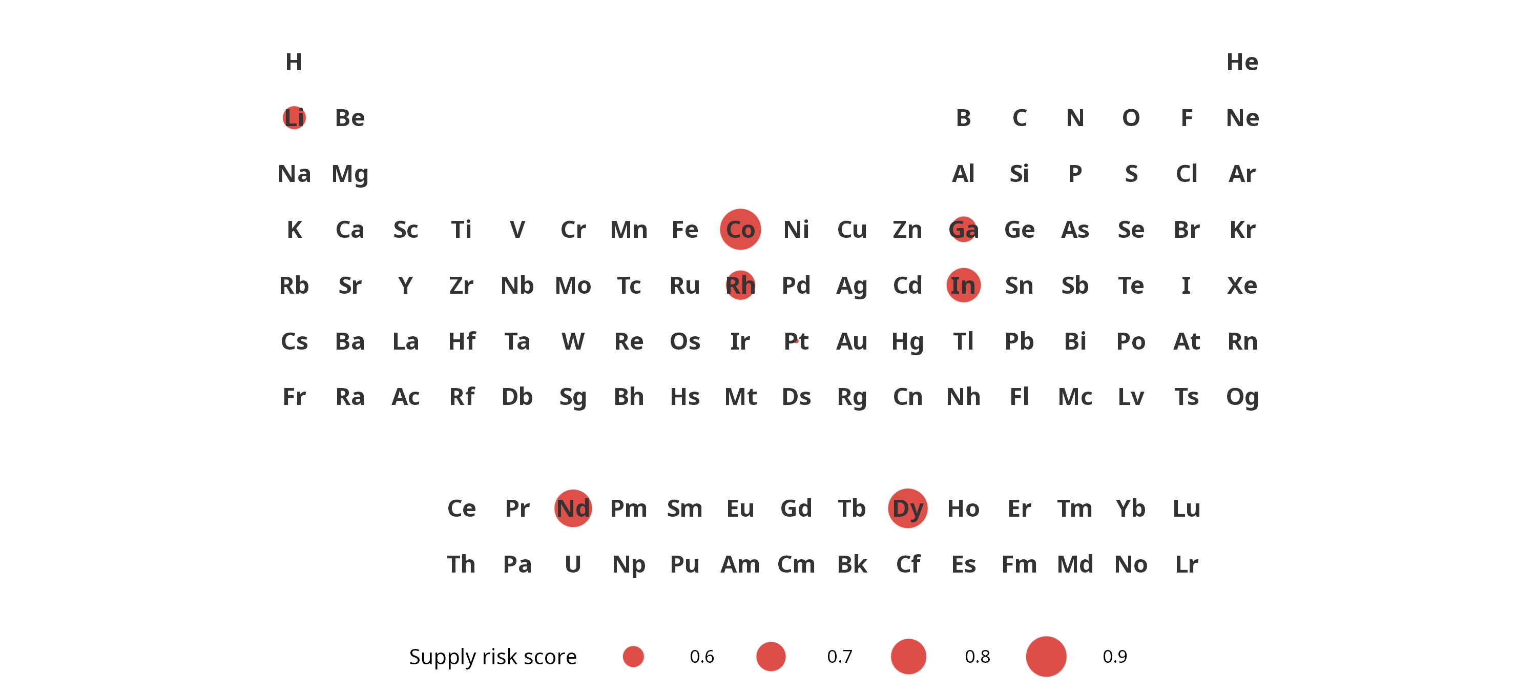
In-tile bar encoding
ggPSE_bar() draws a proportional bar inside each tile
growing from a chosen edge.
ggPSE_bar(supply_risk, value_col = "risk",
          bar_side     = "bottom",
          bar_color    = "#2166ac",
          legend_title = "Supply risk score")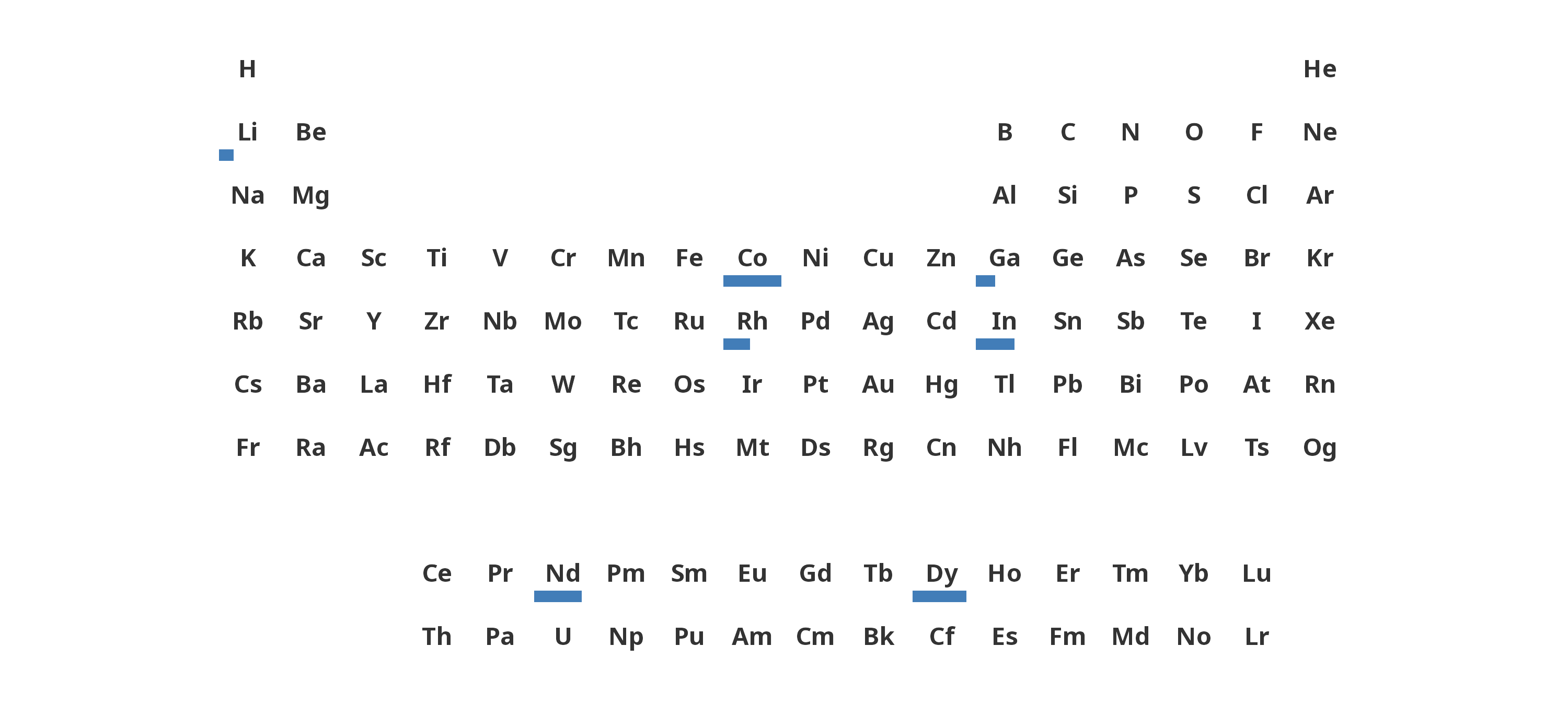
Donut charts per tile
ggPSE_donut() draws a small donut or pie chart inside
each tile showing a categorical breakdown — for example supply mix by
country or phase composition. Requires the ggforce
package.
supply <- data.frame(
  symbol   = c("Li","Li","Li", "Co","Co", "Nd","Nd", "Pt"),
  category = c("CL","AU","AR", "CD","AU", "CN","RU", "ZA"),
  share    = c(0.60, 0.30, 0.10, 0.70, 0.30, 0.80, 0.20, 1.00)
)

ggPSE() |>
  ggPSE_donut(supply, category_col = "category", share_col = "share",
              legend_title = "Producer")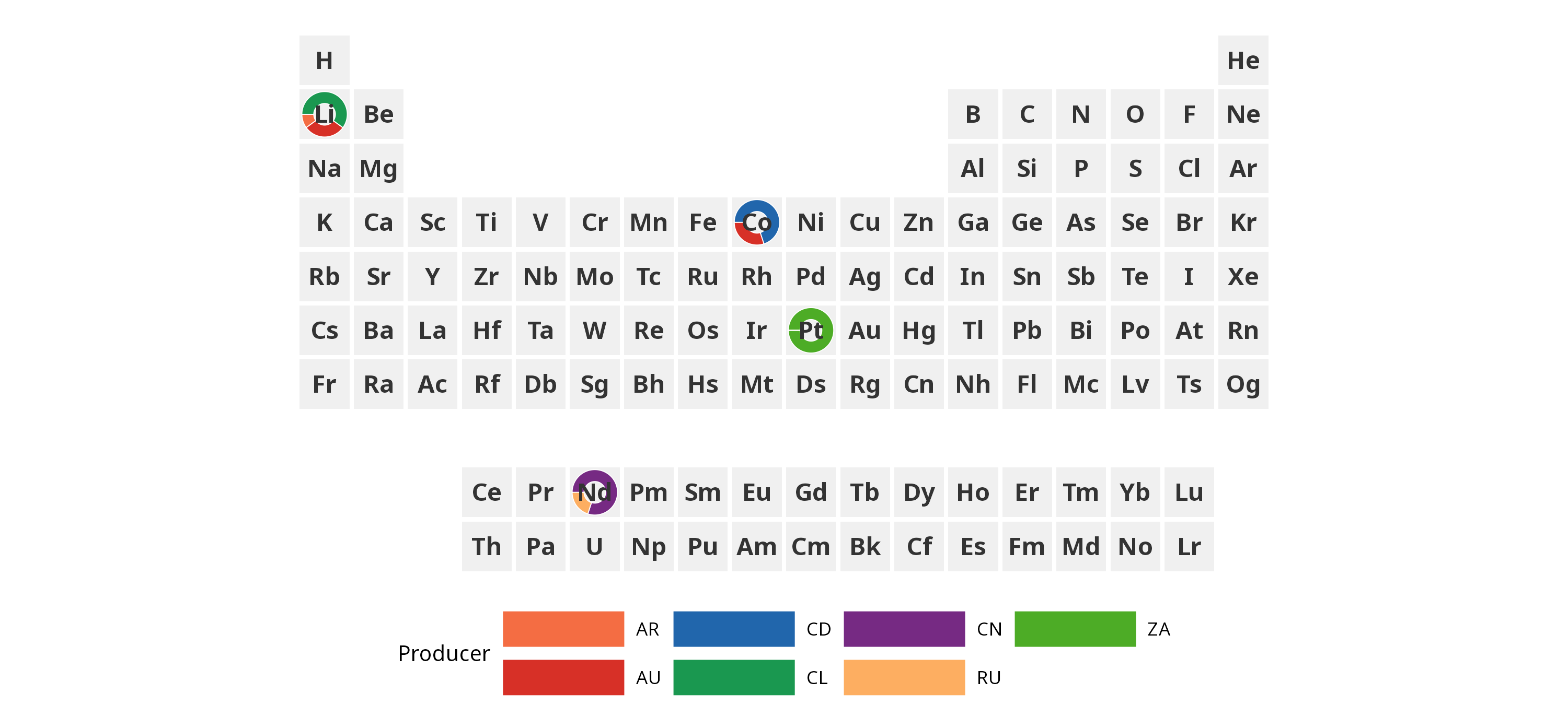
Combine with a gradient fill to encode two variables simultaneously:
# Note: combining gradient fill with donut charts requires ggnewscale
# to avoid scale conflicts - planned for a future release
criticality <- data.frame(
  symbol = c("Li", "Co", "Nd", "Pt"),
  value  = c(0.70, 0.91, 0.85, 0.60)
)
ggPSE(criticality, value_col = "value", legend_title = "Criticality") |>
  ggPSE_donut(supply, category_col = "category", share_col = "share",
              legend_title = "Producer")
Period and group profiles
ggPSE_profile() extracts a single period, group, or
f-block row and combines it with a line plot of a numeric property.
Requires patchwork.
data(ggpse_elements)
ggPSE_profile(ggpse_elements, value_col = "electronegativity", period = 2)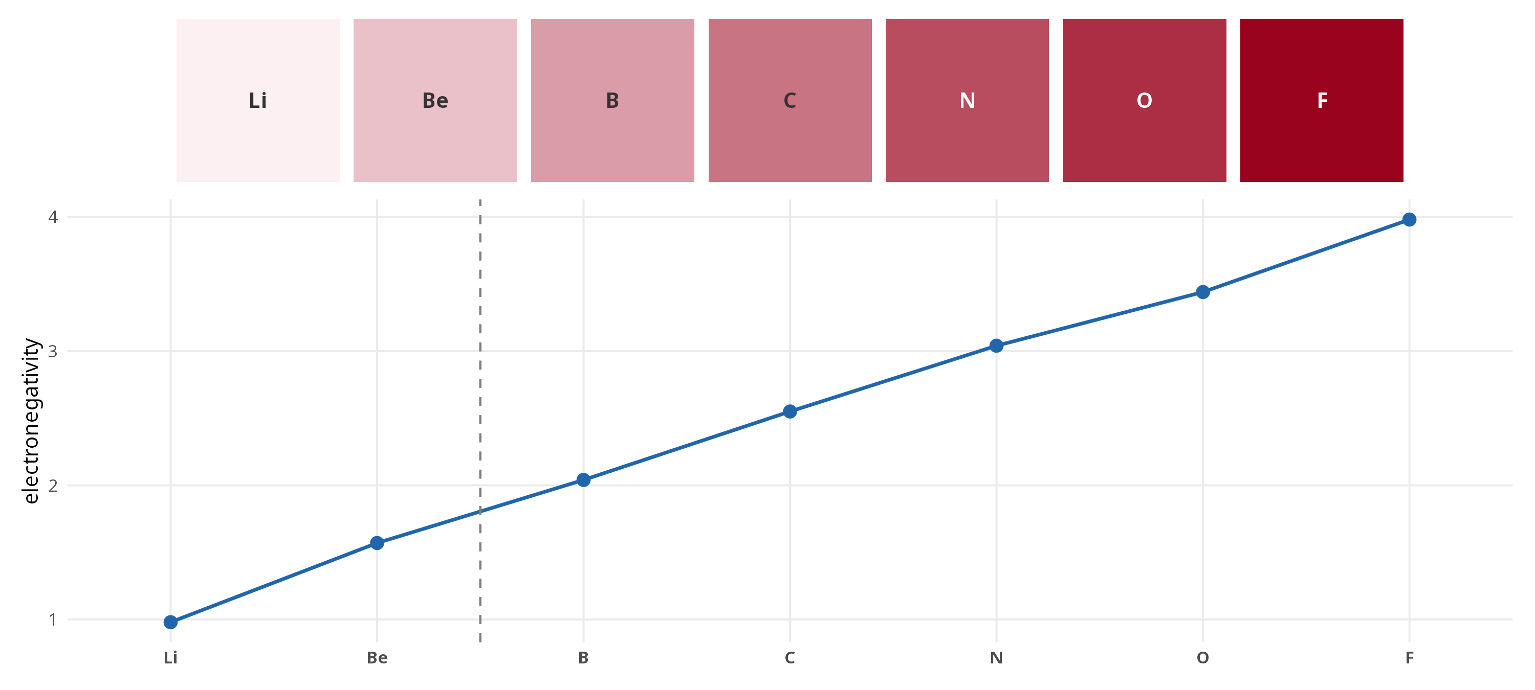
ggPSE_profile(ggpse_elements, value_col = "atomic_radius_pm", group = 1)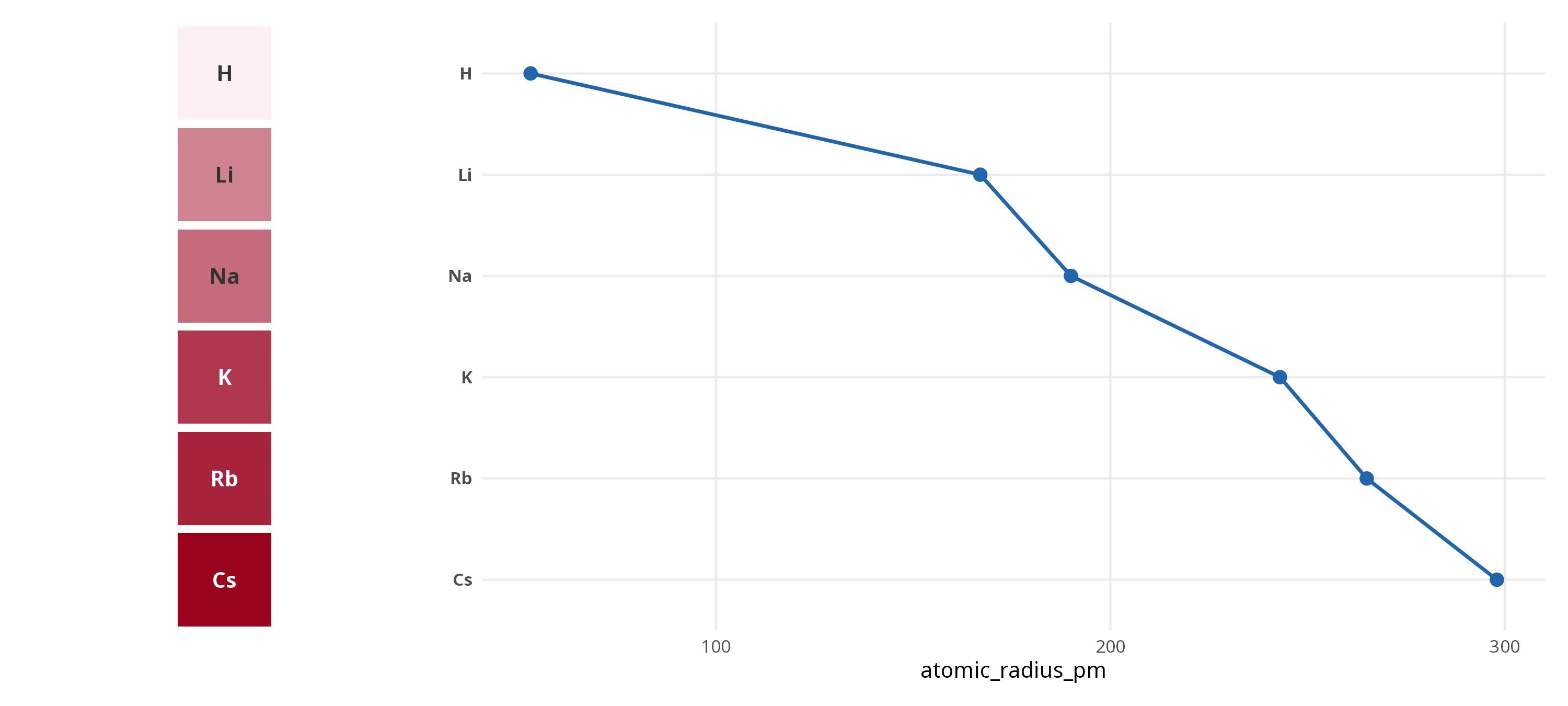
ggPSE_profile(ggpse_elements, value_col = "electronegativity",
              lanthanides = TRUE)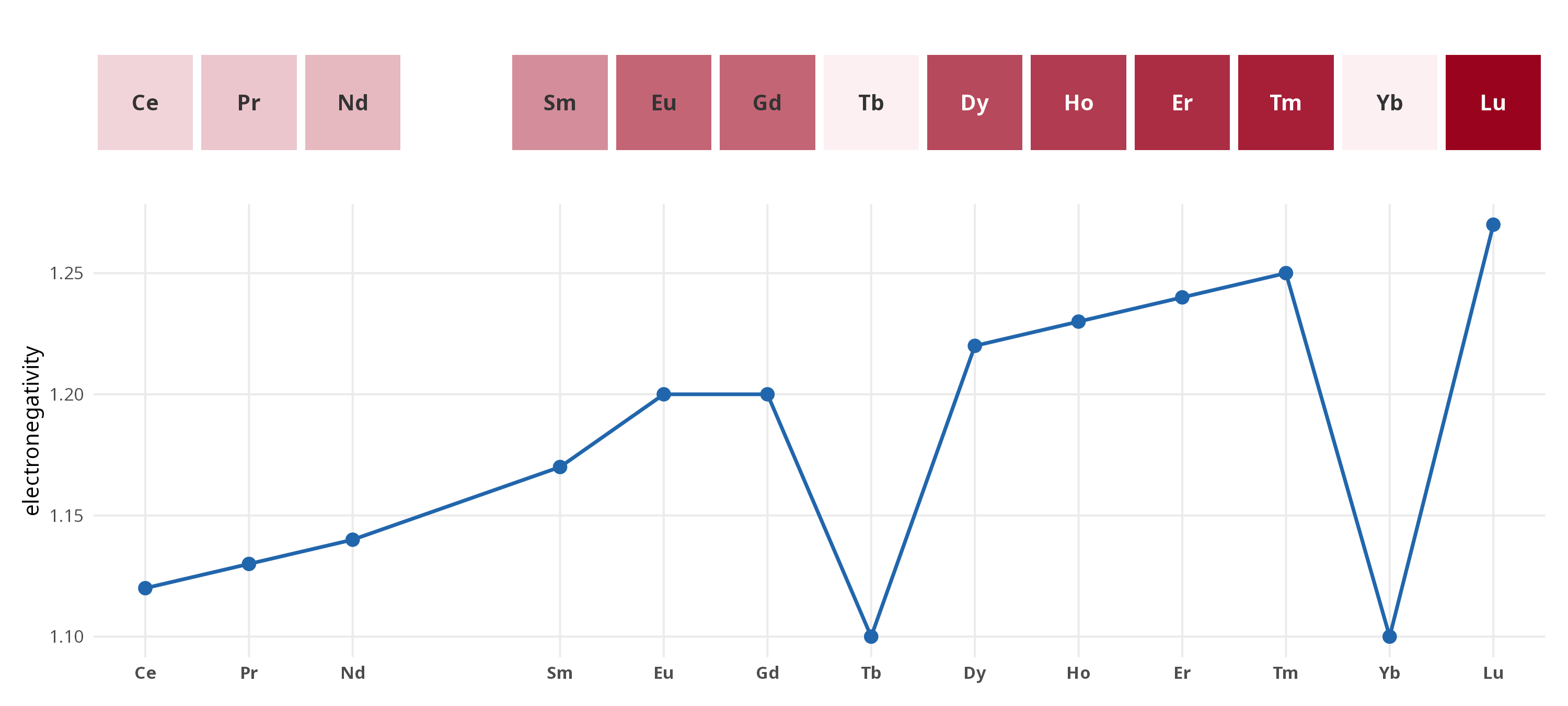
Country-of-origin badges
ggPSE_badge() overlays country flags (via the optional
ggflags package) or ISO 3166-1 alpha-2 text codes. Multiple countries
per element are supported — up to three flags per tile.
supply_single <- data.frame(
  symbol  = c("Li", "Co", "Nd", "Pt", "Cu", "Ni", "Ga", "In"),
  country = c("CL", "CD", "CN", "ZA", "CL", "PH", "CN", "CN"),
  value   = c(0.70, 0.91, 0.85, 0.60, 0.50, 0.55, 0.80, 0.75)
)
ggPSE(supply_single, value_col = "value",
      color_high = "#b2182b", legend_title = "Criticality") |>
  ggPSE_badge(supply_single, country_col = "country")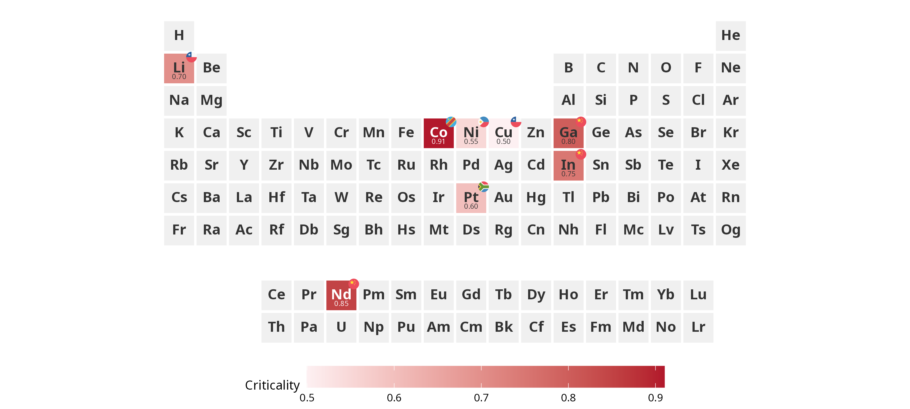
Use hierarchy = TRUE to scale flags by importance order
and show_legend = TRUE to append a country legend. Requires
patchwork.
supply_multi <- data.frame(
  symbol  = c("Li","Li","Li", "Co","Co", "Nd","Nd"),
  country = c("CL","AU","AR", "CD","AU", "CN","RU"),
  value   = c(0.70, 0.70, 0.70, 0.91, 0.91, 0.85, 0.85)
)
ggPSE(supply_multi, value_col = "value", legend_title = "Criticality") |>
  ggPSE_badge(supply_multi, country_col = "country",
              hierarchy = TRUE, show_legend = TRUE)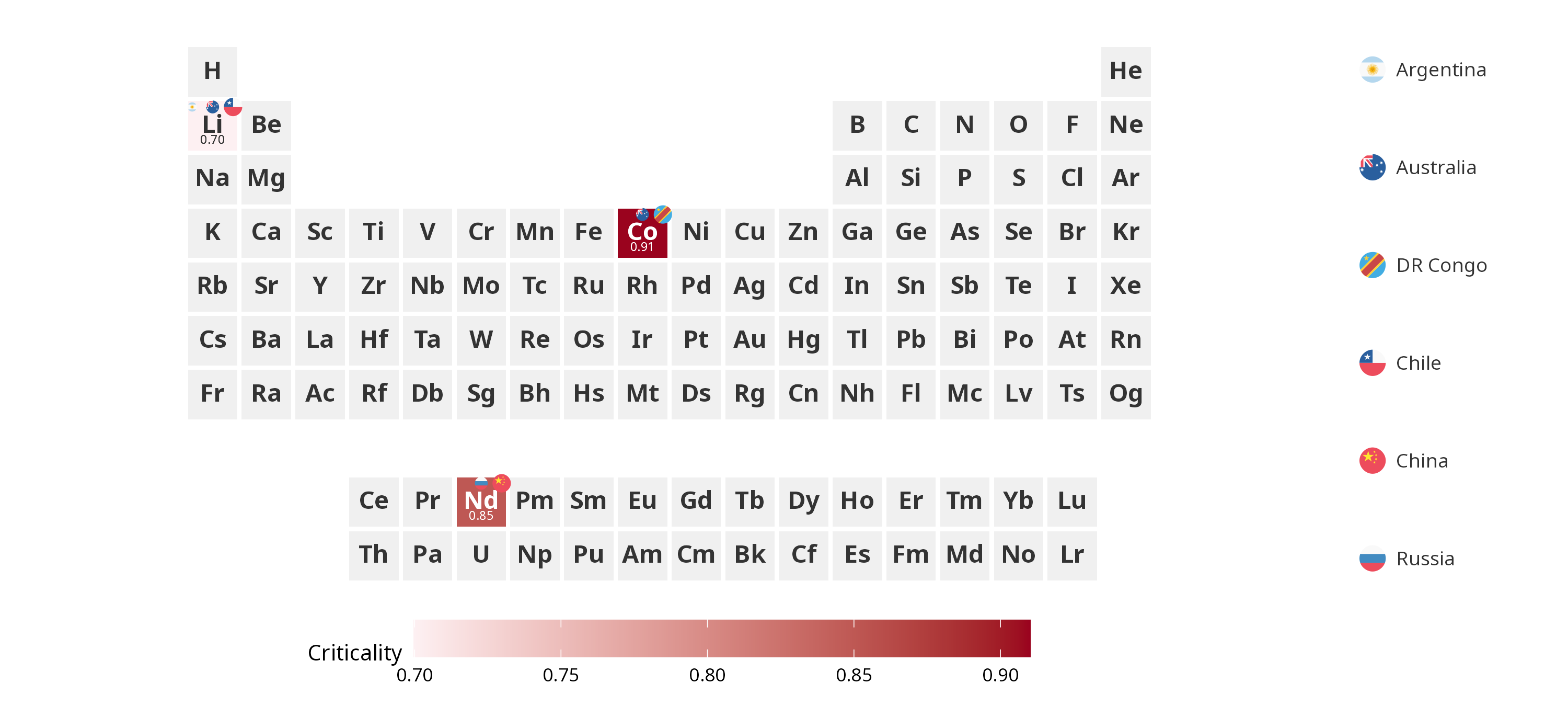
Install ggflags for flag icons:
remotes::install_github("rensa/ggflags")Themes
ggPSE_theme() applies a pre-built visual theme to any
ggPSE plot.
ggPSE(battery, value_col = "importance") |>
  ggPSE_theme("minimal")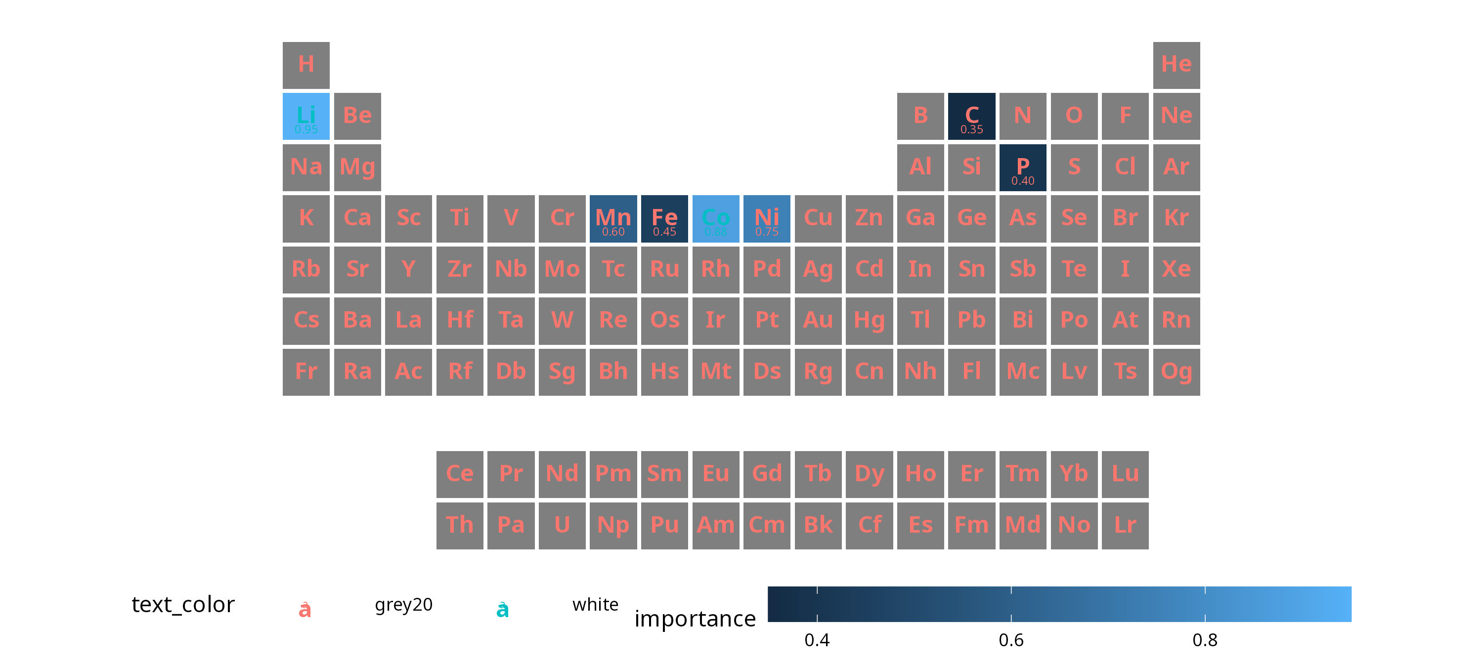
ggPSE(battery, value_col = "importance") |>
  ggPSE_theme("publication")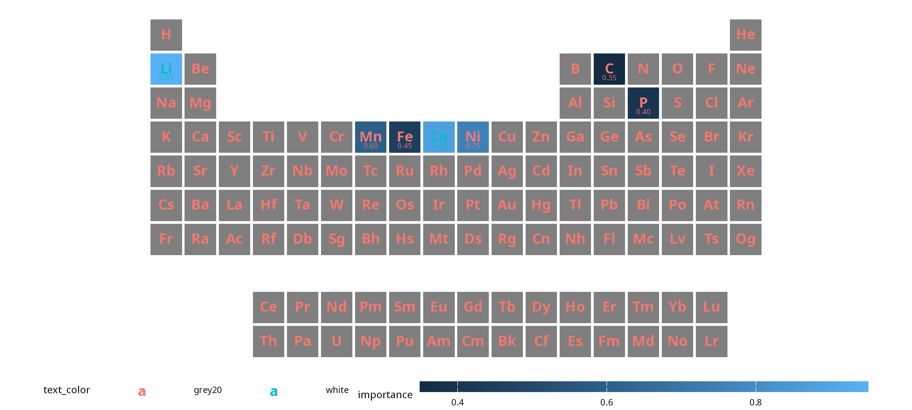
ggPSE() |> ggPSE_theme("crazy", seed = 42)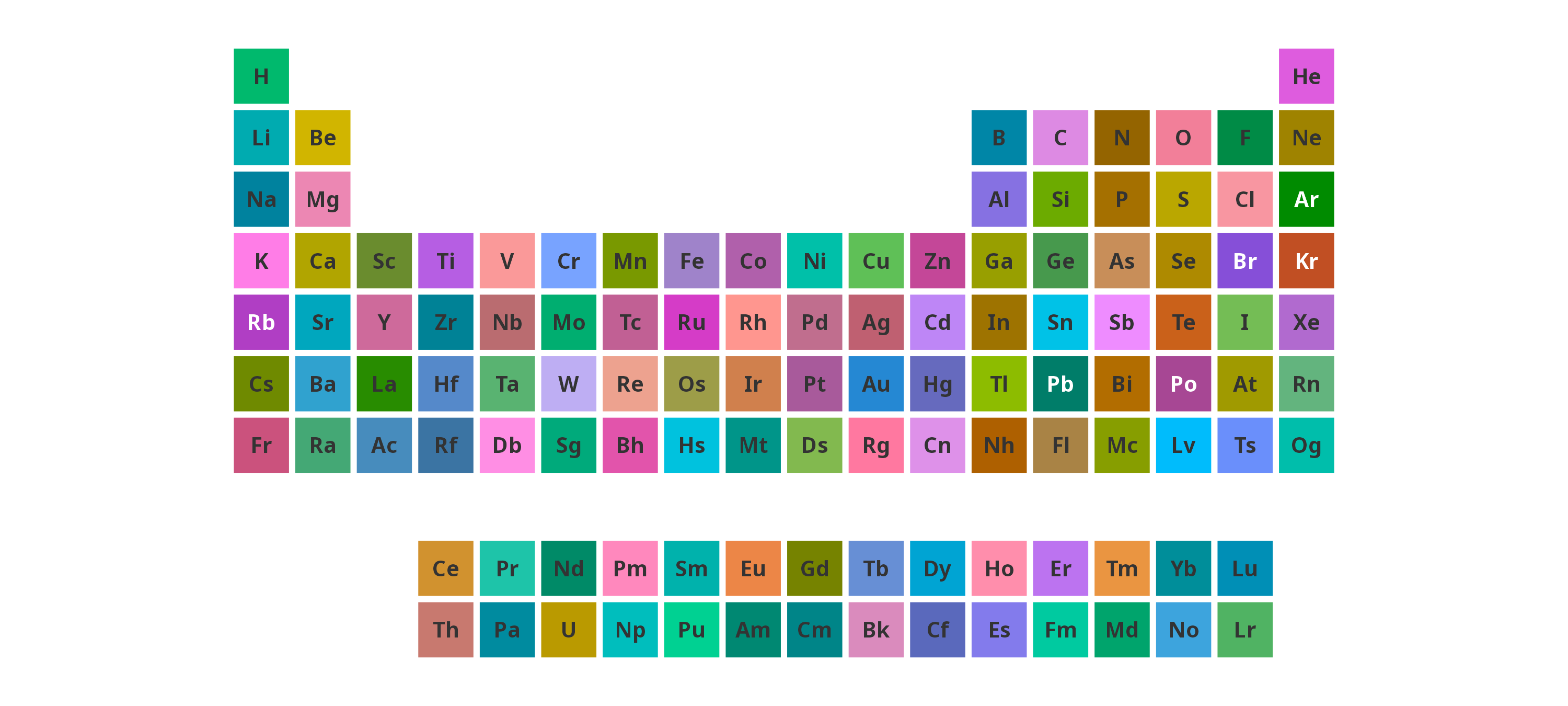
| Theme | Description |
|---|---|
"minimal" |
Clean white background, good for presentations |
"dark" |
Dark plot background with light legend |
"publication" |
Minimal ink, transparent background, journal-ready |
"crazy" |
Random color per tile, reproducible with seed
|
Interactive tooltips
ggPSE_interactive() adds hover tooltips via the
ggiraph package. Renders in HTML documents, Shiny apps, and
RStudio Viewer.
data(ggpse_elements)
ggPSE_interactive(
  ggpse_elements,
  value_col    = "electronegativity",
  tooltip_cols = c("name", "atomic_weight", "block", "electronegativity"),
  legend_title = "Electronegativity (Pauling)"
)
Using the built-in element data
ggPSE ships with ggpse_elements, a data frame of 17
physical and chemical properties for all 118 elements sourced from IUPAC
2021 and NIST WebBook.
data(ggpse_elements)
ggPSE(ggpse_elements, value_col = "electronegativity",
      color_low    = "#f7f7f7",
      color_high   = "#d73027",
      legend_title = "Electronegativity (Pauling)")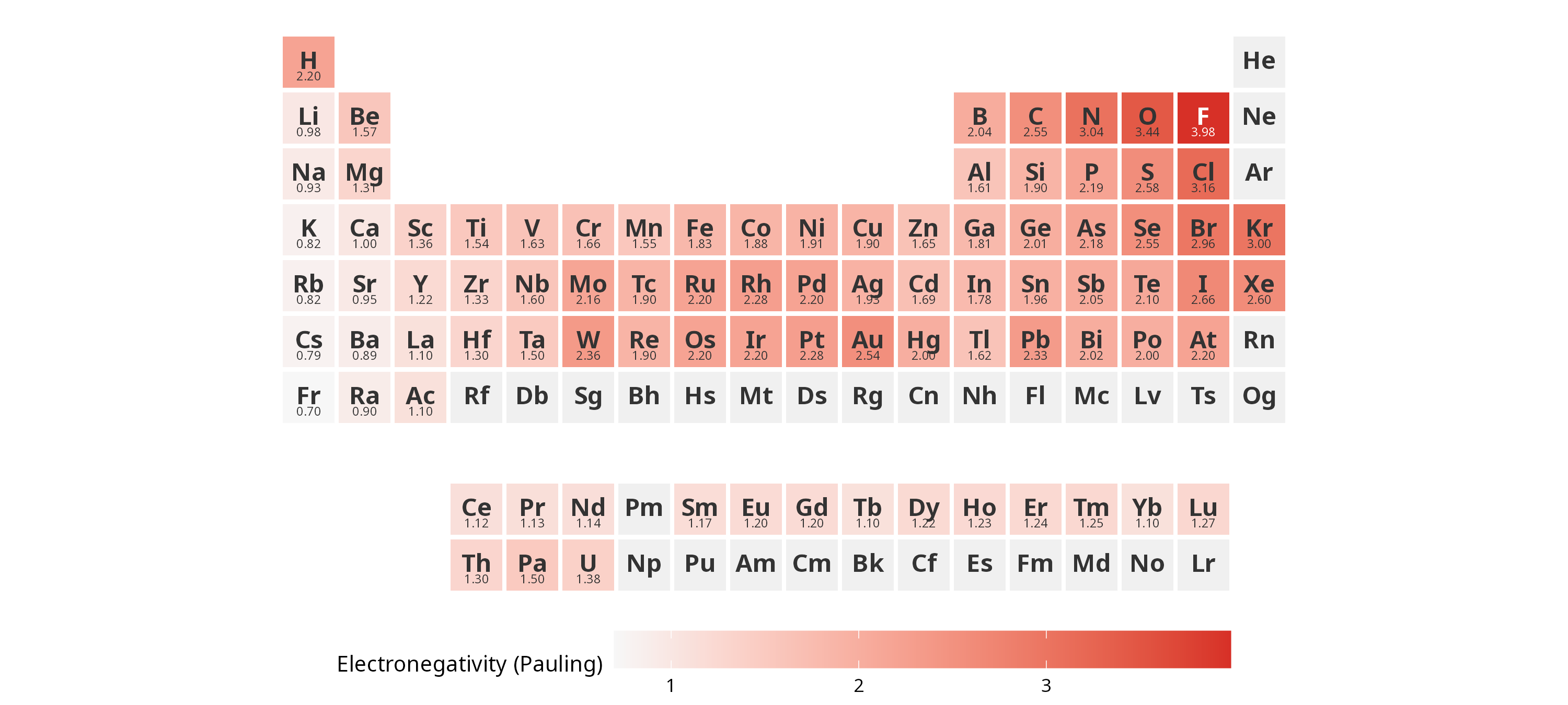
ggPSE(ggpse_elements, value_col = "melting_point_K",
      color_high   = "#08519c",
      legend_title = "Melting point (K)")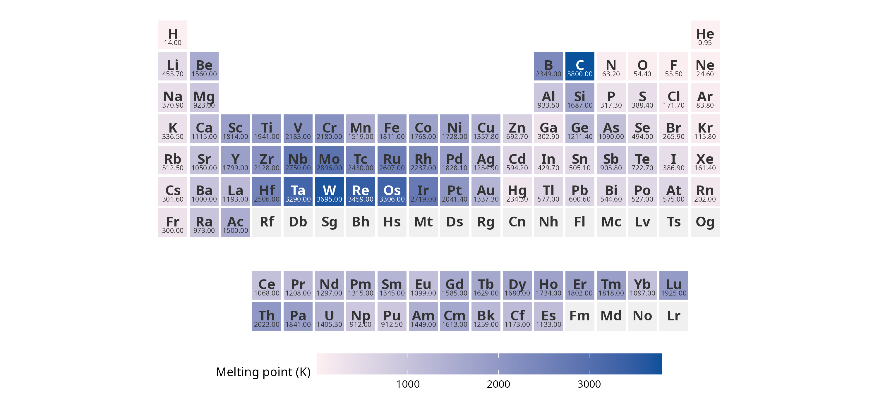
Saving figures
Use ggPSE_save() for sensible periodic table defaults,
or ggsave() directly for full control.
p <- ggPSE(battery, value_col = "importance")

# Convenience wrapper with PSE-optimised defaults
ggPSE_save(p, "battery.png")
ggPSE_save(p, "battery.pdf")

# Full control with ggsave
ggsave("battery.png", p, width = 18, height = 8, units = "cm", dpi = 300)
ggsave("battery.svg", p, width = 18, height = 8, units = "cm")